问题的提出
Example 4.2是一个很接近实际的问题:
Jack管理着一家有两个场地的小型的租车公司(分别称为first location和second location,每租出一部车,Jack可赚10刀。为了提高车子的出租率,Jack在夜间调度车辆,即把车子从一个场地调度到另外一个场地,成本是2刀/辆。假设每个场地每天租车和还车的数量是泊松随机变量,即其数值是n的概率为\(\frac{\lambda^n}{n!}e^{-\lambda}\),其中\(\lambda\)为期望。假设场地1和场地2租车的的\(\lambda\)分别为3和4,还车的\(\lambda\)分别为3和2。为了简化问题起见,我们假设每个场地最多可停20部车(如果归还的车辆超出了20部,我们假设超出的车辆无偿调度到了别的地方,比如总公司),并且每个场地每天最多调度5部车子。
请问Jack在每个场地应该部署多少部车子?每天晚上如何调度?
初步分析
这是每个经营者都关心的问题:利益最大化。部署的车子多了会造成闲置浪费,部署的车子少了会丢掉客户。同样,盲目的调度车辆只会增加调度的费用。
读到这个题目,很自觉的合上书,尝试给出自己的方案。但是说实话,想了半天依然没有很好的头绪。先说一下初步想到的思路:这显然是一个策略优化问题,我们首先要建立策略的模型。对于MDP问题,就是要分析出问题的状态空间、动作空间、状态转移机制(概率)和奖励机制,分别如下:
- 状态空间:两个场地的汽车数量共同决定了一个状态,即问题的状态可以定义为[# of cars of first location, # of cars of second location]。
- 动作空间:在这个问题中有三种动作:租车、还车、调度车辆,哪种动作作为动作空间的元素呢?一时想不清楚……
- 状态转移机制:动作空间没有想清楚,导致状态转移机制也没法考虑:毕竟状态的转移是动作引起的。
- 奖励机制:这个似乎比较明确,
租车的收益-调度的费用即最终的收益作为奖励比较合适。
进一步的分析
进一步的分析发现,虽然租车、还车和调度都会改变状态进而影响最终的收益,但是租车量和还车量是一个我们无法控制的量!只有调度是我们可以控制和优化的量,这也许是问题的核心?
根据问题的假设,调度的上限是5部车子。每调度一部车子,都会对状态空间(两个场地的车子数量)产生影响,进而影响租车的周转率和收益,因此将调度作为一个调优的指标是合理的。那么如何设计调度这个指标呢?
调度是指从一个场地运送车辆到另外一个场地。根据假设,从场地1调度到场地2的车辆数量是[5,-5],其中-5表示从场地2调度5部车到场地1,因此共有11个调度的动作,这就是动作空间。问题转化为对于任意的状态,这11个调度动作如何优化最合理?如下图所示:
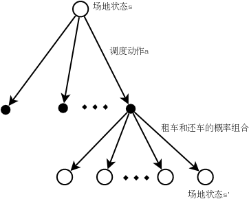
画出了上面这张图,问题应该比较明确了。
程序实现
#######################################################################
# Copyright (C)                                                       #
# 2016 Shangtong Zhang(zhangshangtong.cpp@gmail.com)                  #
# 2016 Kenta Shimada(hyperkentakun@gmail.com)                         #
# 2017 Aja Rangaswamy (aja004@gmail.com)                              #
# 2019 Baochen Su (subaochen@126.com)                                 #
# Permission given to modify the code as long as you keep this        #
# declaration at the top                                              #
#######################################################################

import matplotlib
import matplotlib.pyplot as plt
import numpy as np
import seaborn as sns
from scipy.stats import poisson

matplotlib.use('Agg')

# maximum # of cars in each location
MAX_CARS = 20

# maximum # of cars to move during night
MAX_MOVE_OF_CARS = 5

# expectation for rental requests in first location
REQUEST_FIRST_LOC = 3

# expectation for rental requests in second location
REQUEST_SECOND_LOC = 4

# expectation for # of cars returned in first location
RETURNS_FIRST_LOC = 3

# expectation for # of cars returned in second location
RETURNS_SECOND_LOC = 2

DISCOUNT = 0.9

# credit earned by a car
RENTAL_CREDIT = 10

# cost of moving a car
MOVE_CAR_COST = 2

# all possible actions
actions = np.arange(-MAX_MOVE_OF_CARS, MAX_MOVE_OF_CARS + 1)

# An up bound for poisson distribution
# If n is greater than this value, then the probability of getting n is truncated to 0
# why choose 11 here?
POISSON_UPPER_BOUND = 11

# Probability for poisson distribution
# @lam: lambda should be less than 10 for this function
poisson_cache = dict()


def poisson_probability(n, lam):
    global poisson_cache
    key = n * 10 + lam
    if key not in poisson_cache:
        poisson_cache[key] = poisson.pmf(n, lam)
    return poisson_cache[key]


def expected_return(state, action, state_value, constant_returned_cars):
    """
    @state: [# of cars in first location, # of cars in second location]
    @action: positive if moving cars from first location to second location,
            negative if moving cars from second location to first location
    @stateValue: state value matrix
    @constant_returned_cars:  if set True, model is simplified such that
    the # of cars returned in daytime becomes constant
    rather than a random value from poisson distribution, which will reduce calculation time
    and leave the optimal policy/value state matrix almost the same
    """
    # initialize total return
    returns = 0.0

    # cost for moving cars
    returns -= MOVE_CAR_COST * abs(action)

    # moving cars
    NUM_OF_CARS_FIRST_LOC = min(state[0] - action, MAX_CARS)
    NUM_OF_CARS_SECOND_LOC = min(state[1] + action, MAX_CARS)

    # go through all possible rental requests
    for request_first_loc in range(POISSON_UPPER_BOUND):
        for request_second_loc in range(POISSON_UPPER_BOUND):
            # probability for current combination of rental requests
            prob = poisson_probability(request_first_loc, REQUEST_FIRST_LOC) * \
                poisson_probability(request_second_loc, REQUEST_SECOND_LOC)

            num_of_cars_first_loc = NUM_OF_CARS_FIRST_LOC
            num_of_cars_second_loc = NUM_OF_CARS_SECOND_LOC

            # valid rental requests should be less than actual # of cars
            valid_rental_first_loc = min(num_of_cars_first_loc, request_first_loc)
            valid_rental_second_loc = min(num_of_cars_second_loc, request_second_loc)

            # get credits for renting
            reward = (valid_rental_first_loc + valid_rental_second_loc) * RENTAL_CREDIT
            num_of_cars_first_loc -= valid_rental_first_loc
            num_of_cars_second_loc -= valid_rental_second_loc

            if constant_returned_cars:
                # get returned cars, those cars can be used for renting tomorrow
                returned_cars_first_loc = RETURNS_FIRST_LOC
                returned_cars_second_loc = RETURNS_SECOND_LOC
                num_of_cars_first_loc = min(num_of_cars_first_loc + returned_cars_first_loc, MAX_CARS)
                num_of_cars_second_loc = min(num_of_cars_second_loc + returned_cars_second_loc, MAX_CARS)
                returns += prob * (reward + DISCOUNT * state_value[num_of_cars_first_loc, num_of_cars_second_loc])
            else:
                for returned_cars_first_loc in range(POISSON_UPPER_BOUND):
                    for returned_cars_second_loc in range(POISSON_UPPER_BOUND):
                        prob_return = poisson_probability(returned_cars_first_loc, RETURNS_FIRST_LOC) *\
                            poisson_probability(returned_cars_second_loc, RETURNS_SECOND_LOC)
                        num_of_cars_first_loc_ = min(num_of_cars_first_loc + returned_cars_first_loc, MAX_CARS)
                        num_of_cars_second_loc_ = min(num_of_cars_second_loc + returned_cars_second_loc, MAX_CARS)
                        prob_ = prob_return * prob
                        returns += prob_ * (reward + DISCOUNT *
                                            state_value[num_of_cars_first_loc_, num_of_cars_second_loc_])
    return returns


def figure_4_2(constant_returned_cars=True):
    value = np.zeros((MAX_CARS + 1, MAX_CARS + 1))
    policy = np.zeros(value.shape, dtype=np.int)

    iterations = 0
    _, axes = plt.subplots(2, 3, figsize=(40, 20))
    plt.subplots_adjust(wspace=0.1, hspace=0.2)
    axes = axes.flatten()
    while True:
        fig = sns.heatmap(np.flipud(policy), cmap="YlGnBu", ax=axes[iterations])
        fig.set_ylabel('# cars at first location', fontsize=30)
        fig.set_yticks(list(reversed(range(MAX_CARS + 1))))
        fig.set_xlabel('# cars at second location', fontsize=30)
        fig.set_title('policy {}'.format(iterations), fontsize=30)

        # policy evaluation (in-place)
        while True:
            old_value = value.copy()
            for i in range(MAX_CARS + 1):
                for j in range(MAX_CARS + 1):
                    new_state_value = expected_return([i, j], policy[i, j], value, constant_returned_cars)
                    value[i, j] = new_state_value
            max_value_change = abs(old_value - value).max()
            print('max value change {}'.format(max_value_change))
            if max_value_change < 1e-4:
                break

        # policy improvement
        policy_stable = True
        for i in range(MAX_CARS + 1):
            for j in range(MAX_CARS + 1):
                old_action = policy[i, j]
                action_returns = []
                for action in actions:
                    if (0 <= action <= i) or (-j <= action <= 0):
                        action_returns.append(expected_return([i, j], action, value, constant_returned_cars))
                    else:
                        action_returns.append(-np.inf)
                new_action = actions[np.argmax(action_returns)]
                policy[i, j] = new_action
                if policy_stable and old_action != new_action:
                    policy_stable = False
        print('policy stable {}'.format(policy_stable))

        if policy_stable:
            fig = sns.heatmap(np.flipud(value), cmap="YlGnBu", ax=axes[-1])
            fig.set_ylabel('# cars at first location', fontsize=30)
            fig.set_yticks(list(reversed(range(MAX_CARS + 1))))
            fig.set_xlabel('# cars at second location', fontsize=30)
            fig.set_title('optimal value', fontsize=30)
            break

        iterations += 1

    plt.savefig('../images/rl/dp/figure_4_2.png')
    plt.close()


if __name__ == '__main__':
    figure_4_2()
在理清思路后,上面的代码不难理解,需要重点注意以下几点:
- policy evaluation和policy improvement的迭代过程,这段代码完美的复现了原始算法,值得仔细推敲。
- expeted_return方法看似比较长,其实不难理解,目的是根据\(s,a,v(s)\)计算\(v(s')\)。
完整的程序请参见:car_rental.py
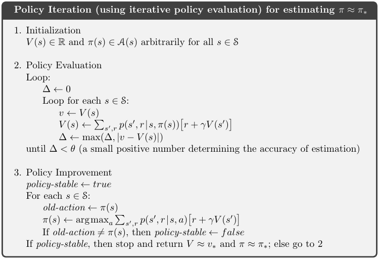
列出policy iteration的算法以对照:
-
Initialization
\(V(s)\in\mathcal{R}\) and \(\pi(s)\in\mathcal{A}\) arbitrarily fro all \(s\in\mathcal{S}\)
-
Policy Evaluation
Loop:
\(\Delta\leftarrow 0\)
loop for each \(s\in\mathcal{S}\):
\(v\leftarrow V(s)\)
\(V(s)\leftarrow \sum_{s',r}p(s',r\mid s,\pi(s))[r+\gamma V(s')]\)
$$\Delta\leftarrow max(\Delta, v-V(s )$$ until \(\Delta<\theta\)(a small positive number determining the accuracy of estimation)
-
Policy Improvement
\[policy\ stable \leftarrow true\]For each \(s\in\mathcal{S}\):
\(old\ action\leftarrow\pi(s)\)
\(\pi(s)\leftarrow argmax_a\sum_{s',r}p(s',r\mid s,a)[r+\gamma v(s')]\)
If \(old\ action \ne \pi(s)\), then \(policy\ stable\leftarrow false\)
If \(policy\ stable\), then stop and return \(V\approx v_*\) and \(\pi\approx \pi_*\); else go to 2
算法描述截图:
结果解读
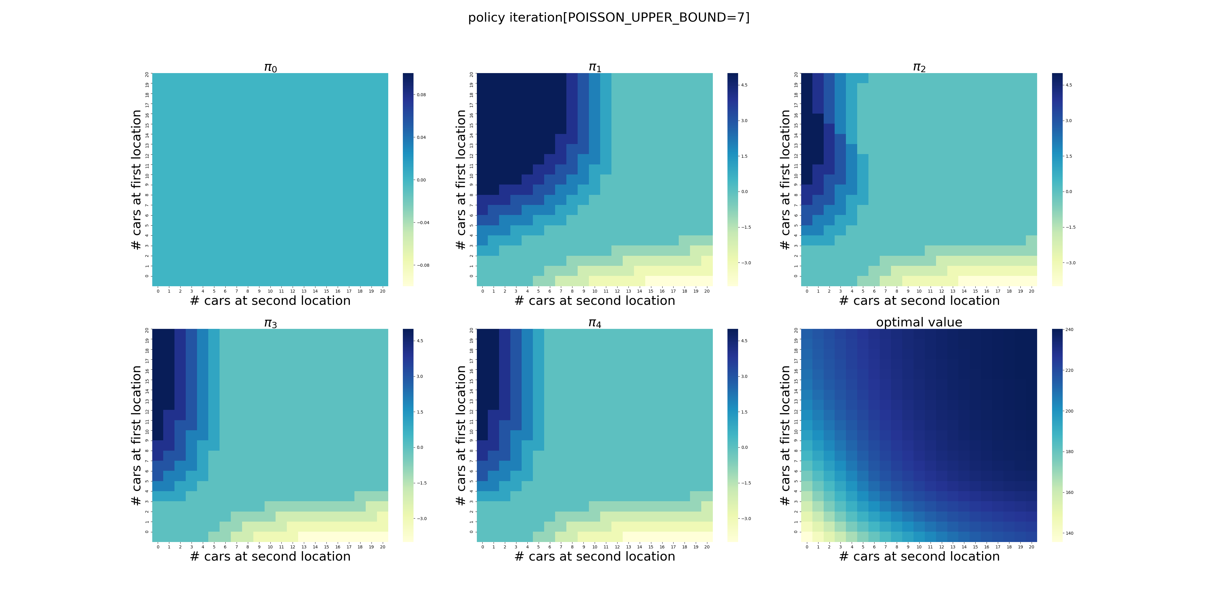
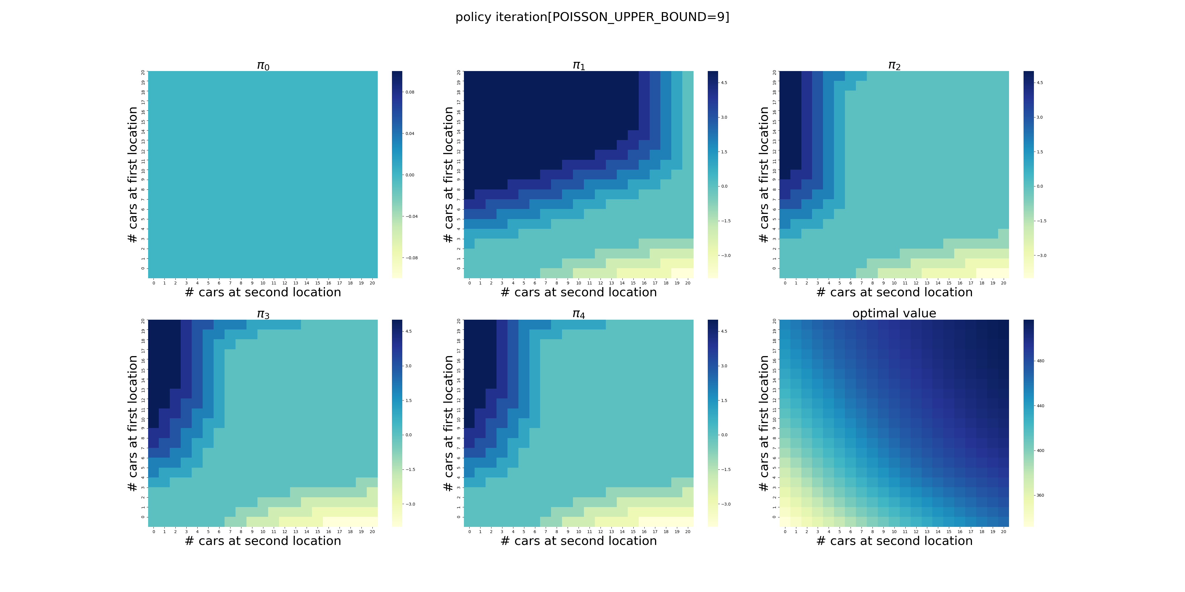
虽然计算量有些大(在我的电脑上耗时2分钟多),但是在有限次的迭代后,程序给出了最优的策略,如下图所示,使用颜色表示了调度车辆的数量(实际上policy3和policy4只有细微的差别,若非最强大脑恐怕都看不出来,反正我没看出来)。在左上角,颜色越深表示调度车辆的数量越大,最深的颜色显然是5辆,依次递减到0辆。在右下角则相反,颜色越浅表示调度的数量越大,依次递增到5辆。
可以看出,当两个场地的车辆数量落在中间的区域时,需要调度的车辆数量为0,显然这是一个动态的过程,需要两个场地的协调和配合,也就是说需要在两个场地之间平衡车辆的数量。
在策略\(\pi_4\)中,我们可以看到场地1的车子数量>3时,可能需要调度;场地2的车子数量>7时,可能需要调度。因此,[3,7]可以看做两个场地的最佳配置。
不过,令我感到困惑的是,当场地1的数量<3,场地2的数量小于<7时,根据\(\pi_4\),显然调度为0,难道意味着无法满足自身需求而无法调度?

进一步的探索
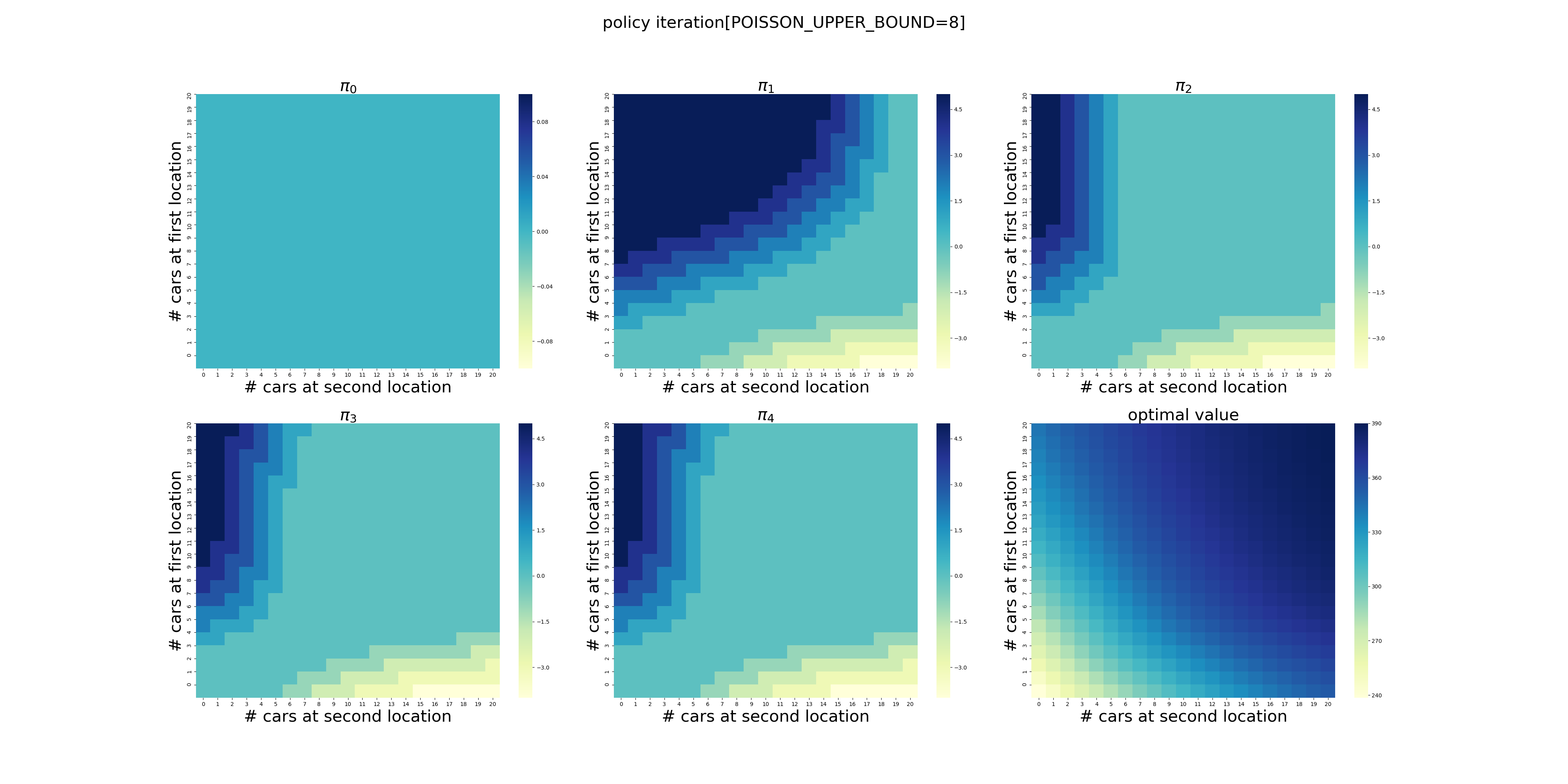
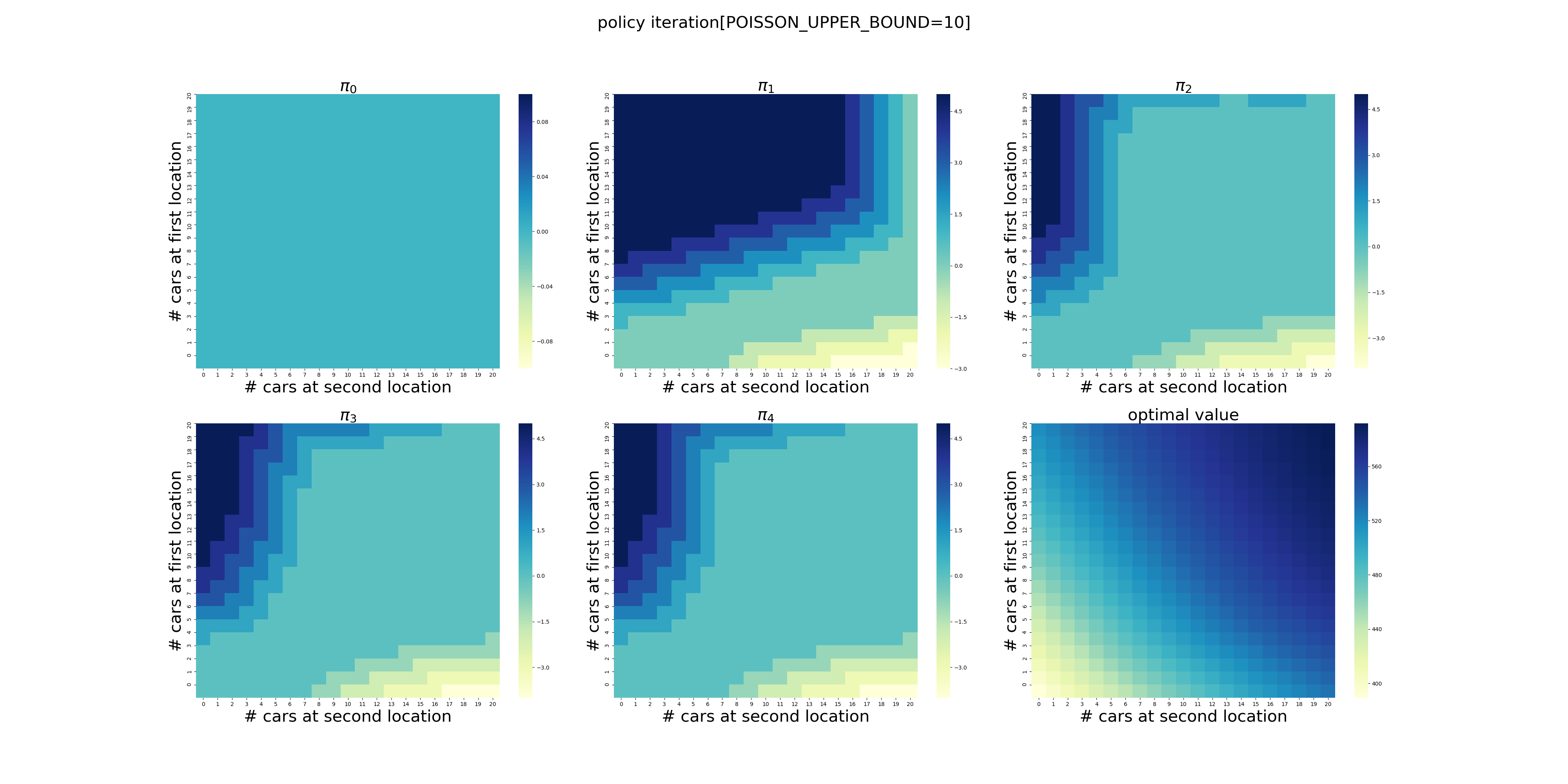
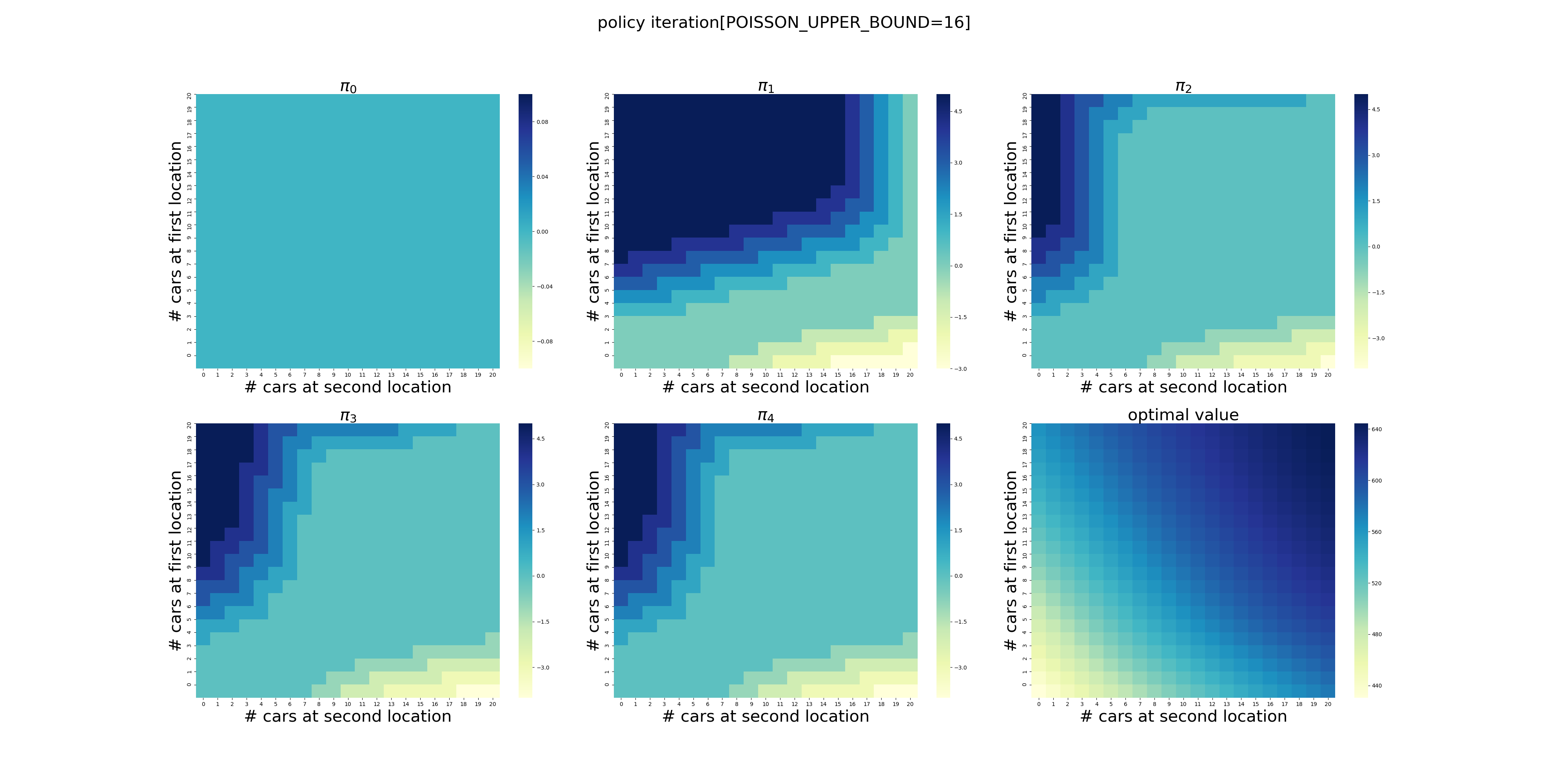
POISSON_UPPER_BOUND的影响
POISSON_UPPER_BOUND在程序里面控制了每个场地最多可以出租/归还多少辆车,超出这个数量强制归0。
下面针对POISSON_UPPER_BOUND在[7,20]区间上进行了计算(耗时56分钟),结果如下。可以看出,在当前的假设条件下,POISSON_UPPER_BOUND>9基本就不会影响最终的结果了,更大的POISSON_UPPER_BOUND设置徒增计算量而已。


更大的车场规模的影响
TBD
更多的停车场
TBD
租车/还车模型的影响
TBD